Standard Costs

When budgets are prepared, the costs are usually computed at two levels, in total dollars so an income statement can be prepared, and cost per unit. The cost per unit is referred to as a standard cost. A standard cost can also be developed and used for pricing decisions and cost control even if a budget is not prepared. A standard cost in a manufacturing company such as Pickup Trucks Company consists of per unit costs for direct materials, direct labor, and overhead. The per unit costs can be further divided into the expected amount and cost of materials per unit, the expected number of hours and cost per hour for direct labor, and the expected total overhead costs and a method for assigning those costs to each unit. Within the expected amount of materials, waste or spoilage must be considered when determining the standard amount. For example, if a product, such as a chair, requires material, more material than is actually needed for the chair must be ordered because the shape of the seat and the fabric are usually not exactly the same. The scraps of material are called waste, which is not avoidable, given that the chair is being produced with this specific fabric. The cost of the full piece of material is used as the standard cost because the waste has no other use.
 

Similarly, when considering labor hours, downtime from production due to maintenance or start up and break time must be included in the number of hours it takes to make a product. Once standards are established, they are used to analyze and determine the reasons for actual cost variances from standards. The variances may be in quantity of materials or hours used to manufacture a product or in the cost of the materials or labor. Because overhead is normally applied on some basis, the variances in overhead will occur because the total overhead pool of dollars or the activity level (for example, direct labor dollars or hours) used to allocate the overhead is different from what was planned. Once standard costs are used in preparing budgets, analysis of variances can be used to provide management with information about whether a variance is caused by quantity or price so that appropriate action can be taken.

To illustrate how cost variance analysis works, assume you are the plant manager for Bases, Inc., a company that makes a set of soft bases for playing baseball in gymnasiums. The budget assumes 150,000 sets of bases will be produced annually. The following standard cost per set of bases was developed:

The predetermined overhead rate of $1.30 will result in $0.65 of overhead being allocated to each set of bases produced. (It is calculated using .5 direct labor hours per set times $1.30 per hour.)

For the month of October, the company produced 13,300 sets of bases. The following information was taken from the October financial report.

Variance Analysis

In order to understand the $1,175 unfavorable monthly variance, it must be analyzed by its component parts: direct materials variances, direct labor variances, and overhead variances. Each of these variances can further be broken down into a price (rate) variance and a quantity (usage or efficiency) variance. A general template that can be used for direct materials variances, direct labor variances, and variable overhead variances uses three amounts — actual, flexible budget, and standard — as a basis for calculating the variances.

The price variance is favorable if actual costs are less than flexible budget costs. The quantity variance is favorable if flexible budget costs are less than standard costs. The total variance is favorable if the actual costs are less than standard costs.

Direct Materials Variances

The total direct materials variance is $2,835 favorable and consists of a $3,000 favorable price variance and a $165 unfavorable quantity variance.

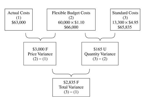
Actual costs of $63,000 are less than flexible budget costs of $66,000, so the materials price variance is $3,000 favorable. The variance can also be thought of on a price per unit basis. The actual costs of $63,000 were for 60,000 feet of direct material, so the actual price per foot is $1.05 ($63,000 ÷ 60,000). The original budget was for a direct materials cost of $1.10 per foot, so it was expected that 60,000 feet of material would cost $66,000. The direct materials actually cost less than budget by $0.05 per foot ($1.10 budget versus $1.05 actual), so the variance is favorable. The direct materials quantity variance of $165 unfavorable means this company used more direct materials than planned because flexible budget costs of $66,000 are higher than the standard costs of $65,825. To produce 13,300 sets of bases, the company expected a cost of $4.95 per set (4.5 feet of material at $1.10 per foot), for a total cost of $65,835. This can also be analyzed by identifying the total feet of material it should have taken to produce 13,300 sets of bases and multiplying by the cost per foot of material (13,300 sets × 4.5 feet per unit = 59,850 feet of direct materials × $1.10 per foot = $65,835). It actually used 60,000 feet, which prices out at an expected $1.10 per foot to be $66,000. The total direct materials variance is calculated by adding the price and quantity variances together or by comparing actual cost of direct materials with the standard cost of producing 13,300 sets of bases.

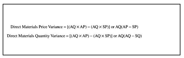
Another way of computing the direct materials variance is using formulas.

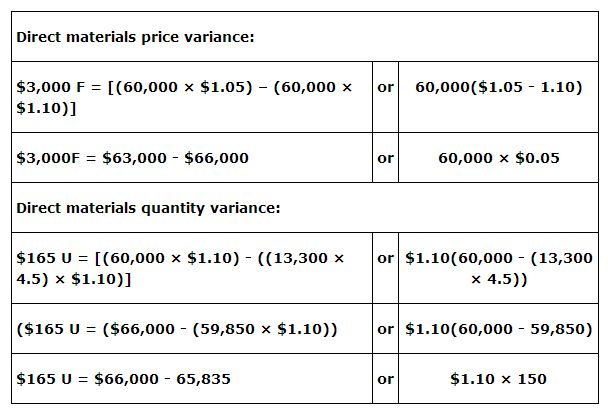
Using the formulas to calculate the variances would work like this:

Once the variances are calculated, management completes the analysis by obtaining explanations for why the variances occurred. For example, a question raised is “Why did materials cost less than planned?” As an answer, management may learn there was a price decrease, or the direct materials were acquired from another source, or lower quality materials were obtained. The explanations for price variances must relate to the cost of the direct materials, not the quantity of the materials used. Similarly, the reasons for the quantity variance need to relate to the amount of materials used, not the price paid for the materials. Reasons for a quantity variance could be more waste or scrap than was planned, or that lower quality materials were used, or less skilled workers were hired or used on the production line, or machine problems occurred that damaged materials.

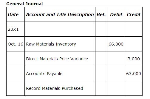
Recording direct materials variances. The direct materials price variance is recorded when the direct materials are purchased. The materials are recorded using actual quantity and standard cost. A separate account is used to track each variance.

The materials quantity variance is recorded when direct materials are requested by production. Direct materials are taken out of raw materials inventory at the same cost they were put in (actual materials quantity at standard price), and work‐in‐process inventory is increased based on the units produced at standard cost.

Direct Labor Variances

The total direct labor variance is $3,525 unfavorable and consists of a $4,875 unfavorable rate variance and a $1,350 favorable efficiency variance. 

Actual labor costs of $63,375 are more than flexible budget costs of $58,500, so the labor rate variance is $4,875 unfavorable. As with materials, the labor can also be thought of on a price per hour basis. The actual costs of $63,375 were for 6,580 hours, which calculates to an average pay rate of $9.75 per direct labor hour. The budget used a rate of $9.00 per direct labor hour. This $0.75 per hour difference resulted in the unfavorable rate variance because actual costs were higher than budgeted costs. This could result from unplanned but negotiated wage rate increases or the use of a more skilled work force.

The efficiency variance is favorable because flexible costs of $58,500 are less than standard costs of $59,850. This means that the employees took less time than budgeted to produce the 13,300 sets of bases. 13,300 units were produced, and the company expected that the labor cost would be $4.50 per set, for a total labor cost of $59,850. This can also be analyzed by identifying the total hours of labor it should have taken to produce 13,300 sets of bases and multiplying by the cost per hour of labor (13,300 sets × .5 hours = 6,650 hours × $9 per hour = $59,850). Because only 6,500 direct labor hours were needed instead of the 6,650 hours expected, the direct labor efficiency variance is favorable.

Recording direct labor variances. The direct labor rate variance is recorded when payroll is accrued.

The direct labor efficiency variance is recorded when the direct labor is assigned to work‐in‐process inventory.

Overhead Variances

Variances may occur for both the variable and fixed cost components of manufacturing overhead. Before looking at the variances, a summary of the overhead information for Bases, Inc., might be helpful. The original plan was for 12,500 units per month, and the actual production for October was 13,300 units.

The variances can be calculated in total for variable and fixed costs, in which case the variances are referred to as the controllable (price) variance and the volume variance. Alternatively, the variances can be calculated separately for variable manufacturing overhead costs and fixed manufacturing overhead costs. The variable overhead cost variances are called the spending (rate) variance and the efficiency variance, and fixed overhead cost variances are known as the spending and volume variances. The variable overhead cost spending variance, the variable overhead cost efficiency variance, and the fixed overhead cost spending variance added together are the same as the controllable variance.

Using the two‐variance approach, the controllable cost variance shows how well management controls its overhead costs. If a volume variance exists, it means the plant operated at a different production level than budgeted. For the Bases, Inc., the total overhead variance is $485 unfavorable. It consists of a $717 unfavorable controllable variance and a $232 favorable volume variance. An unfavorable controllable variance indicates that overhead costs per direct labor hour were higher than expected. The variance is calculated by subtracting the $8,413 budgeted overhead from the $9,130 actual overhead costs. The budgeted overhead is calculated by adding budgeted variable costs for the actual number of units (think of this as the flexible budget amount) to the budgeted fixed costs (unchanged from original budget).

For Bases, Inc., production was 13,300 units and variable costs were $0.72 per direct labor hour. As each unit takes .5 direct labor hours to make, the variable overhead is 13,300 units times .5 hours times $0.72, or $4,788. When added to fixed costs of $3,625, the total budgeted overhead costs are $8,413 for the month. Possible reasons for the unfavorable variance are: indirect materials were purchased from a different supplier with higher costs, or more indirect materials were used due to waste; indirect labor rates were higher due to a change in personnel or higher negotiated raises than budgeted; and/or fixed overhead costs were more than budgeted.

The $232 volume variance indicates an over‐application of fixed costs. This occurred because actual production is higher than the budget. Remember that as more units are produced, fixed costs per unit decrease. However, the predetermined overhead rate is established when the budget is prepared, and the same rate is used throughout the year regardless of the actual number of units produced. So even though the fixed costs per unit decreased when 13,300 units were produced rather than the 12,500 budgeted, the same predetermined overhead rate using the higher cost per unit was used to allocate overhead to production.

Using the separate overhead variance calculations for variable and fixed costs, the total overhead variance is the same $485 unfavorable. The total variable overhead cost variance is $542 unfavorable, indicating actual variable costs were higher than standard variable costs and, therefore, the overhead is underapplied. The total fixed overhead variance is $57 favorable, indicating overhead is overapplied, because the actual fixed costs are less than the standard fixed costs.

The $650 unfavorable variable cost spending variance is calculated by subtracting the $4,680 flexible budget for variable overhead (actual direct labor hours times variable overhead per direct labor hour, or 6,500 × $0.72) from the actual variable overhead of $5,330. It is unfavorable because more was spent on variable overhead costs per direct labor hour than the $0.72 that was budgeted. Knowing that total variable costs are $5,330 and that 6,500 direct labor hours were incurred, the actual variable overhead costs per direct labor hour rate was $0.82. The $108 favorable efficiency variance is determined by subtracting $4,788 standard overhead (13,300 units by the variable overhead per unit predetermined rate of $0.36) from the flexible budget variable overhead cost of $4,680. It occurred because it took only 6,500 direct labor hours instead of 6,650 (13,300 units × .5 hours per unit) direct labor hours to produce the 13,300 units. The total variable cost variance of $542 is calculated by adding the $650 unfavorable spending variance and the $108 favorable efficiency variance.

The $175 unfavorable fixed cost spending variance indicates more was spent on fixed costs than was budgeted. It is calculated by subtracting the budgeted fixed overhead per month of $3,625 from the $3,800 actual fixed overhead. The $232 favorable volume variance indicates fixed overhead costs are overapplied. This occurred because there were more units produced than planned. It is calculated by subtracting the applied fixed overhead based on standard cost for units produced of $3,857 (13,300 sets × $0.29 per unit) from budgeted fixed overhead of $3,625. The total fixed overhead cost variance of $57 favorable is the combination of the $175 unfavorable spending variance and the $232 favorable volume variance.

When combined together, the variable overhead spending variance, the variable overhead efficiency variance, and the fixed cost spending variance equal the $717 unfavorable controllable variance calculated under the two‐variance method previously discussed.

Recording overhead variances. As manufacturing overhead is incurred, it is recorded in the manufacturing overhead account. The entry to record the variable and fixed components of manufacturing overhead is:

Manufacturing overhead is applied to production based on direct labor hours.


At the end of the period, overhead variances are recognized. Under the two variance methods, the entry is:


Once these entries are recorded, the manufacturing overhead account is zero.

Using the second method described for manufacturing overhead variances, the entry to record the overhead variances would be:

Total Variance

The $1,175 total unfavorable variance has now been analyzed into its components for further follow‐up by management:

The balances in the variance accounts are usually closed to the cost of goods sold account, particularly when the amounts are small. Alternatively, the balances in the variance accounts may be allocated to the appropriate inventory accounts and the cost of goods sold account.


Back to Top
×
A18ACD436D5A3997E3DA2573E3FD792A