The way a specific cost reacts to changes in activity levels is called cost behavior. Costs may stay the same or may change proportionately in response to a change in activity. Knowing how a cost reacts to a change in the level of activity makes it easier to create a budget, prepare a forecast, determine how much profit a new product will generate, and determine which of two alternatives should be selected.
Fixed costs
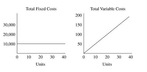
Fixed costs are those that stay the same in total regardless of the number of units produced or sold. Although total fixed costs are the same, fixed costs per unit changes as fewer or more units are produced. Straight‐line depreciation is an example of a fixed cost. It does not matter whether the machine is used to produce 1,000 units or 10,000,000 units in a month, the depreciation expense is the same because it is based on the number of years the machine will be in service.
Variable costs
Variable costs are the costs that change in total each time an additional unit is produced or sold. With a variable cost, the per unit cost stays the same, but the more units produced or sold, the higher the total cost. Direct materials is a variable cost. If it takes one yard of fabric at a cost of $5 per yard to make one chair, the total materials cost for one chair is $5. The total cost for 10 chairs is $50 (10 chairs × $5 per chair) and the total cost for 100 chairs is $500 (100 chairs × $5 per chair).
Graphically, the total fixed cost looks like a straight horizontal line while the total variable cost line slopes upward.
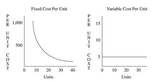
The graphs for the fixed cost per unit and variable cost per unit look exactly opposite the total fixed costs and total variable costs graphs. Although total fixed costs are constant, the fixed cost per unit changes with the number of units. The variable cost per unit is constant.
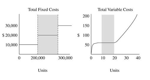
When cost behavior is discussed, an assumption must be made about operating levels. At certain levels of activity, new machines might be needed, which results in more depreciation, or overtime may be required of existing employees, resulting in higher per hour direct labor costs. The definitions of fixed cost and variable cost assumes the company is operating or selling within the relevant range (the shaded area in the graphs) so additional costs will not be incurred.
Mixed costs
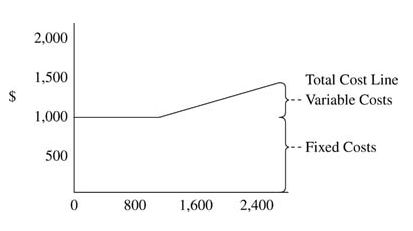
Some costs, called mixed costs, have characteristics of both fixed and variable costs. For example, a company pays a fee of $1,000 for the first 800 local phone calls in a month and $0.10 per local call made above 800. During March, a company made 2,000 local calls. Its phone bill will be $1,120 ($1,000 +(1,200 × $0.10)).
To analyze cost behavior when costs are mixed, the cost must be split into its fixed and variable components. Several methods, including scatter diagrams, the high‐low method, and least‐square regression, are used to identify the variable and fixed portions of a mixed cost, which are based on the past experience of the company.
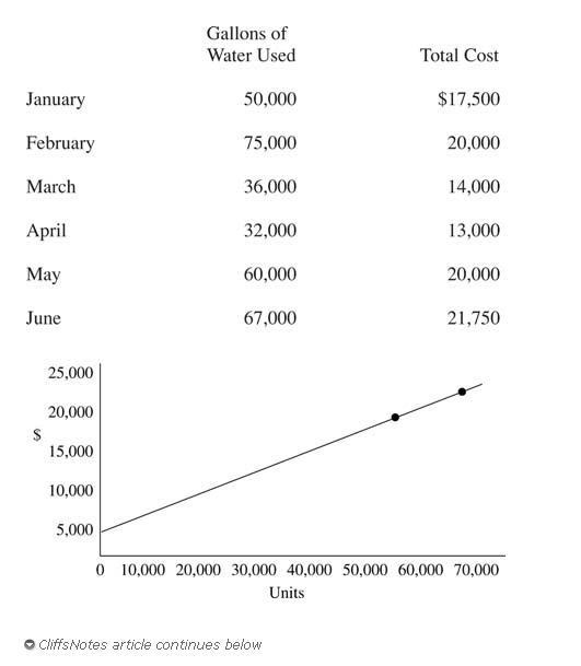
Scatter diagram. In a scatter diagram, all parts would be plotted on a graph with activity (gallons of water used, in the example graph later in this section) on the horizontal axis and cost on the vertical axis. A line is drawn through the points and an estimate made for total fixed costs at the point where the line intersects the vertical axis at zero units of activity. To compute the variable cost per unit, the slope of the line is determined by choosing two points and dividing the change in their cost by the change in the units of activity for the two points selected.
For example, using data from the following example, if 36,000 gallons of water and 60,000 gallons of water were selected, the change in cost is $6,000 ($20,000 – $14,000) and the change in activity is 24,000 (60,000 – 36,000). This makes the slope of the line, the variable cost, $0.25 ($6,000 ÷ 24,000), and the fixed costs $5,000. See the graph to illustrate the point.
High‐low method. The high‐low method divides the change in costs for the highest and lowest levels of activity by the change in units for the highest and lowest levels of activity to estimate variable costs. The high point of activity is 75,000 gallons and the low point is 32,000 gallons. The variable cost per unit is estimated to be $0.163. It was calculated by dividing $7,000 ($20,000 – $13,000) by 43,000 (75,000 – 32,000) gallons of water.
Least‐squares regression analysis. The least‐squares regression analysis is a statistical method used to calculate variable costs. It requires a computer spreadsheet program (for example, Excel) or calculator and uses all points of data instead of just two points like the high‐low method.