Requirements: Normally distributed population, σ is unknown
Test for population mean
Hypothesis test
Formula: 
where  is the sample mean, Δ is a specified value to be tested, s is the sample standard deviation, and n is the size of the sample. Look up the significance level of the z-value in the standard normal table (Table 2 in "Statistics Tables").
When the standard deviation of the sample is substituted for the standard deviation of the population, the statistic does not have a normal distribution; it has what is called the t‐distribution(see Table 3 in "Statistics Tables"). Because there is a different t‐distribution for each sample size, it is not practical to list a separate area‐of ‐the‐curve table for each one. Instead, critical t‐values for common alpha levels (0.10, 0.05, 0.01, and so forth) are usually given in a single table for a range of sample sizes. For very large samples, the t‐distribution approximates the standard normal ( z) distribution. In practice, it is best to use t‐distributions any time the population standard deviation is not known.
Values in the t‐table are not actually listed by sample size but by degrees of freedom (df). The number of degrees of freedom for a problem involving the t‐distribution for sample size n is simply n – 1 for a one‐sample mean problem.
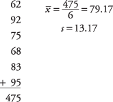
A professor wants to know if her introductory statistics class has a good grasp of basic math. Six students are chosen at random from the class and given a math proficiency test. The professor wants the class to be able to score above 70 on the test. The six students get scores of 62, 92, 75, 68, 83, and 95. Can the professor have 90 percent confidence that the mean score for the class on the test would be above 70?
null hypothesis: H 0: μ = 70
alternative hypothesis: H a : μ > 70
First, compute the sample mean and standard deviation:
Next, compute the t‐value:
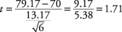
To test the hypothesis, the computed t‐value of 1.71 will be compared to the critical value in the t‐table. But which do you expect to be larger and which do you expect to be smaller? One way to reason about this is to look at the formula and see what effect different means would have on the computation. If the sample mean had been 85 instead of 79.17, the resulting t‐value would have been larger. Because the sample mean is in the numerator, the larger it is, the larger the resulting figure will be. At the same time, you know that a higher sample mean will make it more likely that the professor will conclude that the math proficiency of the class is satisfactory and that the null hypothesis of less‐than‐satisfactory class math knowledge can be rejected. Therefore, it must be true that the larger the computed t‐value, the greater the chance that the null hypothesis can be rejected. It follows, then, that if the computed t‐value is larger than the critical t‐value from the table, the null hypothesis can be rejected.
A 90 percent confidence level is equivalent to an alpha level of 0.10. Because extreme values in one rather than two directions will lead to rejection of the null hypothesis, this is a one‐tailed test, and you do not divide the alpha level by 2. The number of degrees of freedom for the problem is 6 – 1 = 5. The value in the t‐table for t .10,5 is 1.476. Because the computed t‐value of 1.71 is larger than the critical value in the table, the null hypothesis can be rejected, and the professor has evidence that the class mean on the math test would be at least 70.
Note that the formula for the one‐sample t‐test for a population mean is the same as the z‐test, except that the t‐test substitutes the sample standard deviation s for the population standard deviation σ and takes critical values from the t‐distribution instead of the z‐distribution. The t‐distribution is particularly useful for tests with small samples ( n < 30).
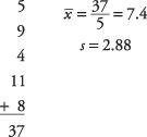
A Little League baseball coach wants to know if his team is representative of other teams in scoring runs. Nationally, the average number of runs scored by a Little League team in a game is 5.7. He chooses five games at random in which his team scored 5 , 9, 4, 11, and 8 runs. Is it likely that his team's scores could have come from the national distribution? Assume an alpha level of 0.05.
Because the team's scoring rate could be either higher than or lower than the national average, the problem calls for a two‐tailed test. First, state the null and alternative hypotheses:
null hypothesis: H 0: μ = 5.7
alternative hypothesis: H a : μ ≠ 5.7
Next compute the sample mean and standard deviation:
Next, the t‐value:
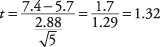
Now, look up the critical value from the t‐table(Table 3 in "Statistics Tables"). You need to know two things in order to do this: the degrees of freedom and the desired alpha level. The degrees of freedom is 5 – 1 = 4. The overall alpha level is 0.05, but because this is a two‐tailed test, the alpha level must be divided by two, which yields 0.025. The tabled value for t .025,4is 2.776. The computed t of 1.32 is smaller, so you cannot reject the null hypothesis that the mean of this team is equal to the population mean. The coach cannot conclude that his team is different from the national distribution on runs scored.
Formula: 
where a and b are the limits of the confidence interval,  is the sample mean,
  is the value from the t‐table corresponding to half of the desired alpha level at n – 1 degrees of freedom, s is the sample standard deviation, and n is the size of the sample.
Using the previous example, what is a 95 percent confidence interval for runs scored per team per game?
First, determine the t‐value. A 95 percent confidence level is equivalent to an alpha level of 0.05. Half of 0.05 is 0.025. The t‐value corresponding to an area of 0.025 at either end of the t‐distribution for 4 degrees of freedom ( t .025,4) is 2.776. The interval may now be calculated:
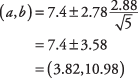
The interval is fairly wide, mostly because n is small.