To describe the linear association between quantitative variables, a statistical procedure called regression often is used to construct a model. Regression is used to assess the contribution of one or more “explanatory” variables (called independent variables) to one “response” (or dependent) variable. It also can be used to predict the value of one variable based on the values of others. When there is only one independent variable and when the relationship can be expressed as a straight line, the procedure is called simple linear regression.
Figure 1. A straight line.

Returning to the exercise example, you observed that the scatter plot of points in Figure
resembles a line. The regression procedure fits the best possible straight line to an array of data points. If no single line can be drawn such that all the points fall on it, what is the “best” line? Statisticians use the line that minimizes the sum of squared deviations from each data point to the line, a fact that will become clearer after you compute the line for the example.
Regression is an inferential procedure, meaning that it can be used to draw conclusions about populations based on samples randomly drawn from those populations. Suppose that your ten exercise‐machine owners were randomly selected to represent the population of all exercise‐machine owners. In order to use this sample to make educated guesses about the relationship between the two variables (months of machine ownership and time spent exercising) in the population, you need to rewrite the equation above to reflect the fact that you will be estimating population parameters:
y = β 0 + β 1 x
All you have done is replace the intercept ( a) with β 0 and the slope (b) with β 1. The formula to compute the parameter estimate  is
is 
where 
and 
The formula to compute the parameter estimate  is
is 
where  and
and  are the two sample means.
You already have computed the quantities that you need to substitute into these formulas for the exercise example—except for the  mean of
  , which is
  , and the
  mean of
  , which is
  . First, compute the estimate of the slope:
Now the intercept may be computed: 
So, the regression equation for the example is y = 9.856 – 0.665 x. When you plot this line over the data points, the result looks like that shown in Figure 2.
Figure 2. Illustration of residuals.

The vertical distance from each data point to the regression line is the error, or residual, of the line's accuracy in estimating that point. Some points have positive residuals (they lie above the line); some have negative ones (they lie below it). If all the points fell on the line, there would be no error and no residuals. The mean of the sample residuals is always 0 because the regression line is always drawn such that half of the error is above it and half below it. The equations that you used to estimate the intercept and slope determine a line of “best fit” by minimizing the sum of the squared residuals. This method of regression is called least squares.
Because regression estimates usually contain some error (that is, all points do not fall on the line), an error term (ε, the Greek letter epsilon) is usually added to the end of the equation:
y = β 0 + β 1 x + ε
The estimate of the slope β 1 for the exercise example was –0.665. The slope is negative because the line slants down from left to right, as it must for two variables that are negatively correlated, reflecting that one variable decreases as the other increases. When the correlation is positive, β 1is positive, and the line slants up from left to right.
Confidence interval for the slope
Example 1
What if the slope is 0, as in Figure 3? That means that y has no linear dependence on x, or that knowing x does not contribute anything to your ability to predict y.
It is often useful to compute a confidence interval for a regression slope. If it contained 0, you would be unable to conclude that x and y are related. The formula to compute a confidence interval for β 1 is 
where 
and 
and where  is the sum of the squared residuals,
  is the critical value from the t‐table corresponding to half the desired alpha level at n – 2 degrees of freedom, and n is the size of the sample (the number of data pairs). The test for this example will use an alpha of 0.05. Table 3 (in "Statistics Tables") shows that t .025,8 = 2.306.
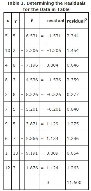
Compute the quantity  by subtracting each predicted y‐value
  from each actual y‐value, squaring it, and summing the squares (see Table 1). The predicted y‐value
  is the y‐value that would be predicted from each given x, using the formula y = 9.856 – 0.665 x.
Now, compute s: 
You have already determined that S xx = 110.4; you can proceed to the main formula: 
You can be 95 percent confident that the population parameter β 1 (the slope) is no lower than –0.929 and no higher than –0.401. Because this interval does not contain 0, you would be able to reject the null hypothesis that β 1 = 0 and conclude that these two variables are indeed related in the population.
Figure 3. An example of uncorrelated data, so the slope is zero.

Confidence interval for prediction
You have learned that you could predict a y‐value from a given x‐value. Because there is some error associated with your prediction, however, you might want to produce a confidence interval rather than a simple point estimate. The formula for a prediction interval for y for a given x is 
where 
and 
and where  is the y‐value predicted for x using the regression equation,
  is the critical value from the t‐table corresponding to half the desired alpha level at n – 2 degrees of freedom, and n is the size of the sample (the number of data pairs).
What is a 90 percent confidence interval for the number of hours spent exercising per week if the exercise machine is owned 11 months?
The first step is to use the original regression equation to compute a point estimate for y: 
For a 90 percent confidence interval, you need to use t .05,8, which Table 3 (in "Statistics Tables") shows to be 1.860. You have already computed the remaining quantities, so you can proceed with the formula: 
You can be 90 percent confident that the population mean for the number of hours spent exercising per week when x (number of weeks machine owned) = 11 is between about 0 and 5.
Assumptions and cautions
The use of regression for parametric inference assumes that the errors (ε) are (1) independent of each other and (2) normally distributed with the same variance for each level of the independent variable. Figure 4 shows a violation of the second assumption. The errors (residuals) are greater for higher values of x than for lower values.
Figure 4. Data with increasing variance as x increases.

Least squares regression is sensitive to outliers, or data points that fall far from most other points. If you were to add the single data point x = 15, y = 12 to the exercise data, the regression line would change to the dotted line shown in Figure 5. You need to be wary of outliers because they can influence the regression equation greatly.
Figure 5. Least squares regression is sensitive to outliers.

It can be dangerous to extrapolate in regression—to predict values beyond the range of your data set. The regression model assumes that the straight line extends to infinity in both directions, which often is not true. According to the regression equation for the example, people who have owned their exercise machines longer than around 15 months do not exercise at all. It is more likely, however, that “hours of exercise” reaches some minimum threshold and then declines only gradually, if at all (see Figure 6).
Figure 6. Extrapolation beyond the data is dangerous.

|
|
|
|
|
|
|
|
|
|