Statistics

A probability distribution is a pictorial display of the probability— P( x) —for any value of x. Consider the number of possible outcomes of two coins being flipped (see Table 1). Table 2 shows the probability distribution of the results of flipping two coins. Figure 1 displays this information graphically.

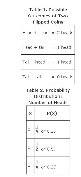
Figure 1.Probability distribution of the results of flipping two coins.

Discrete versus continuous variables

The number of heads resulting from coin flips can be counted only in integers (whole numbers). The number of aces drawn from a deck can be counted only in integers. These “countable” numbers are known as discrete variables: 0, 1, 2, 3, 4, and so forth. Nothing in between two variables is possible. For example, 2.6 is not possible.

Qualities such as height, weight, temperature, distance, and so forth, however, can be measured using fractions or decimals as well: 34.27, 102.26, and so forth. These are known as continuous variables.

Total of probabilities of discrete variables

The probability of a discrete variable lies somewhere between 0 and 1, inclusive. For example, the probability of tossing one head in two coin flips is, as earlier, 0.50. The probability of tossing two heads in two coin flips is 0.25, and the probability of tossing no heads in two coin flips is 0.25. The sum (total) of probabilities for all values of x always equals 1. For example, note that in Tables 1 and 2, adding the probabilities for all the possible outcomes yields a sum of 1.