Solving Differential Equations
You can use the Laplace transform operator to solve (first‐ and second‐order) differential equations with constant coefficients. The differential equations must be IVP's with the initial condition (s) specified at x = 0.
The method is simple to describe. Given an IVP, apply the Laplace transform operator to both sides of the differential equation. This will transform the differential equation into an algebraic equation whose unknown, F(p), is the Laplace transform of the desired solution. Once you solve this algebraic equation for F( p), take the inverse Laplace transform of both sides; the result is the solution to the original IVP.
Before this process is undertaken, it is necessary to see what the Laplace transform operator does to y′ and y″. Integration by parts yields
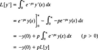
so
Replacing y by y′ in this result gives the Laplace transform of y″:
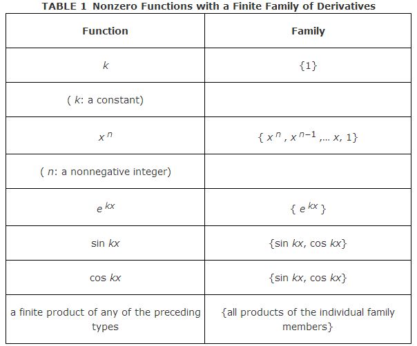
Table 1 assembles the Laplace transforms of a few of the most frequently encountered functions, as well as some of the important properties of the Laplace transform operator L.
Example 1: Use the Laplace transform operator to solve the IVP

Apply the operator L to both sides of the differential equation; then use linearity, the initial condition, and Table 1 to solve for L[ y]:
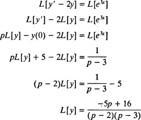
Therefore,
By partial fraction decomposition,
so
is the solution of the IVP.
Usually when faced with an IVP, you first find the general solution of the differential equation and then use the initial condition (s) to evaluate the constant(s) By contrast, the Laplace transform method uses the initial conditions at the beginning of the solution so that the result obtained in the final step by taking the inverse Laplace transform automatically has the constants evaluated.
Example 2: Use Laplace transforms to solve
Apply the operator L to both sides of the differential equation; then use linearity, the initial conditions, and Table 1 to solve for L[ y]:
But the partial fraction decompotion of this expression for L[ y] is
Therefore,
which yields

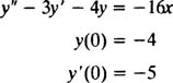
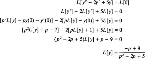
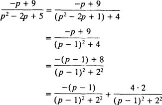
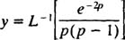
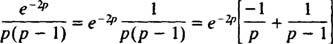
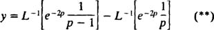
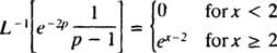
Example 3: Use Laplace transforms to determine the solution of the IVP
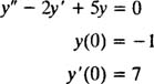
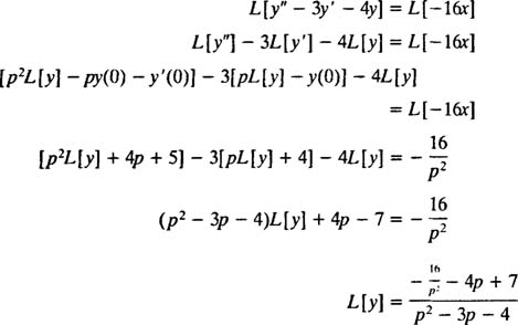
Apply the operator L to both sides of the differential equation; then use linearity, the initial conditions, and Table 1 to solve for L[ y]
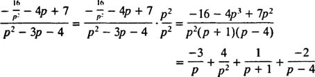
Now,
so
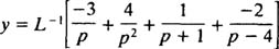
or more simply,

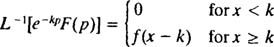
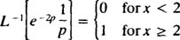
Example 4: Use the fact that if f( x) = −1[ F ( p)], then for any positive constant k,
to solve and sketch the solution of the IVP

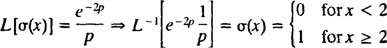
where σ is the step function
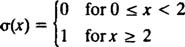
shown in Figure 1.

Figure 1
The Laplace transform method is particularly well‐suited to solving IVP's that involve discontinuous functions such as the previously shown step function σ.
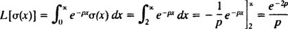
As usual, begin by taking the Laplce of both sides of the differential equation:

Since y (0) = 0, the left‐hand side of (*) reduces to

Using the definition of L, the right‐hand side of (*) is now evaluated:
Therefore, the transformed equation (*) reads
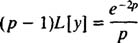
so
But
so
Now, Since L −1[1/( p – 1)] = e x , the formula given in the statement of the problem says
and since L −1[1/( p] = 1), applying the formula given in the statement of the problem again yields
Alternatively, simply notice that
Substituting these results into (**) gives the solution of the IVP:
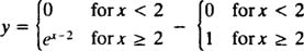
which becomes
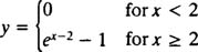
This function is sketched in Figure 2:

|
|
|
|
|
|
|
|
|
|
|
Figure 2