The general second‐order homogeneous linear differential equation has the form

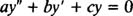
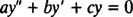
If a( x), b( x), and c( x) are actually constants, a( x) ≡ a ≠ 0, b( x) ≡ b, c( x) ≡ c, then the equation becomes simply
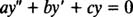
This is the general second‐order homogeneous linear equation with constant coefficients.
Theorem A above says that the general solution of this equation is the general linear combination of any two linearly independent solutions. So how are these two linearly independent solutions found? The following example will illustrate the fundamental idea.
Example 1: Solve the differential equation y″ – y′ – 2 y = 0.
The trick is to substitute y = e mx ( m a constant) into the equation; you will see shortly why this approach works. If y = e mx , then y′ = me mx and y″ = m 2 e mx , so the differential equation becomes

The term e mx can be factored out and immediately canceled (since e mx never equals zero):
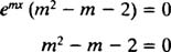
This quadratic polynomial equation can be solved by factoring:
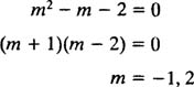
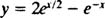
Now, recall that the solution began by writing y = e mx . Since the values of m have now been found m = −1, m = 2), both 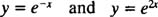 are solutions. Since these functions are linearly independent (neither is a constant multiple of the other), Theorem A says that the general linear combination
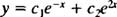
is the general solution of the differential equation.
Note carefully that the solution of the homogeneous differential equation
depends entirely on the roots of the auxiliary polynomial equation that results from substituting y = e mx and then canceling out the e mx term. Once the roots of this auxiliary polynomial equation are found, you can immediately write down the general solution of the given differential equation. Also note that a second‐order linear homogeneous differential equation with constant coefficients will always give rise to a second‐degree auxiliary polynomial equation, that is, to a quadratic polynomial equation.
The roots of any quadratic equation

are given by the famous quadratic formula
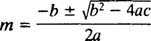
The quantity under the square root sign, b 2 – 4 ac, is called the discriminant of the equation, and its sign determines the nature of the roots. There are exactly three cases to consider.
Case 1: The discriminant is positive.
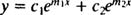
In this case, the roots are real and distinct. If the two roots are denoted m 1 and m 2, then the general solution of the differential equation is
Case 2: The discriminant is zero.
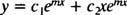
In this case, the roots are real and identical; that is, the polynomial equation has a double (repeated) root. If this double root is denoted simply by m, then the general solution of the differential equation is
Case 3: The discriminant is negative.
In this case, the roots are distinct conjugate complex numbers, r ± si. The general solution of the differential equation is then

So here's the process: Given a second‐order homogeneous linear differential equation with constant coefficients ( a ≠ 0),
immediately write down the corresponding auxiliary quadratic polynomial equation

(found by simply replacing y″ by m 2, y′ by m, and y by 1). Determine the roots of this quadratic equation, and then, depending on whether the roots fall into Case 1, Case 2, or Case 3, write the general solution of the differential equation according to the form given for that Case.
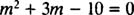
Example 2: Solve the differential equation y″ + 3 y′ – 10 y = 0.
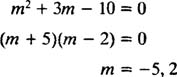
The auxiliary polynomial equation is
whose roots are real and distinct:
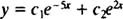
This problem falls into Case 1, so the general solution of the differential equation is
Example 3: Give the general solution of the differential equation y″ – 2 y′ + y = 0.
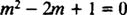
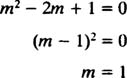
The auxiliary polynomial equation is
which has a double root:
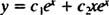
This problem falls into Case 2, so the general solution of the differential equation is
Example 4: Solve the differential equation y″ – 6 y′ + 25 y = 0.
The auxiliary quadratic equation is
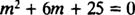
which has distinct conjugate complex roots:

This problem falls into Case 3, so the general solution of the differential equation is

Example 5: Solve the IVP
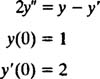
First, rewrite the differential equation in standard form:
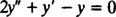
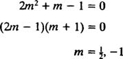
Next, form the auxiliary polynomial equation
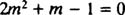
and determine its roots:
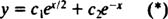
Since the roots are real and distinct, this problem falls into Case 1, and the general solution of the differential equation is therefore
All that remains is to use the two given initial conditions to determine the values of the constants c 1 and c 2:
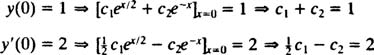
These two equations for c 1 and c 2 can be solved by first adding them to yield
then substituting c 1 = 2 back into either equation to find c 2 = −1.
From (*), the solution of the given IVP is therefore