First-Order Linear Equations
A first‐order differential equation is said to be linear if it can be expressed in the form
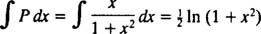
where P and Q are functions of x. The method for solving such equations is similar to the one used to solve nonexact equations. There, the nonexact equation was multiplied by an integrating factor, which then made it easy to solve (because the equation became exact).
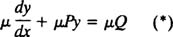
To solve a first‐order linear equation, first rewrite it (if necessary) in the standard form above; then multiply both sides by the integrating factor

The resulting equation,
is then easy to solve, not because it's exact, but because the left‐hand side collapses:
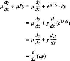
Therefore, equation (*) becomes

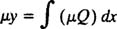
making it susceptible to an integration, which gives the solution:
Do not memorize this equation for the solution; memorize the steps needed to get there.
Example 1: Solve the differential equation

The equation is already expressed in standard form, with P(x) = 2 x and Q(x) = x. Multiplying both sides by
transforms the given differential equation into
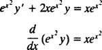
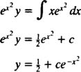
Notice how the left‐hand side collapses into ( μy)′; as shown above, this will always happen. Integrating both sides gives the solution:
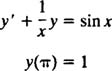
Example 2: Solve the IVP
Note that the differential equation is already in standard form. Since P(x) = 1/ x, the integrating factor is

Multiplying both sides of the standard‐form differential equation by μ = x gives
Note how the left‐hand side automatically collapses into ( μy)′. Integrating both sides yields the general solution:
Applying the initial condition y(π) = 1 determines the constant c:

Thus the desired particular solution is
or, since x cannot equal zero (note the coefficient P(x) = 1/ x in the given differential equation),
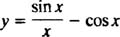
Example 3: Solve the linear differential equation

First, rewrite the equation in standard form:
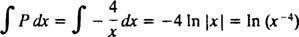
Since the integrating factor here is

multiply both sides of the standard‐form equation (*) by μ = e −2/ x ,
collapse the left‐hand side,
and integrate:

Thus the general solution of the differential equation can be expressed explicitly as 
Example 4: Find the general solution of each of the following equations:
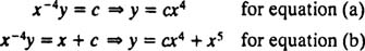
a. 
b. 
Both equations are linear equations in standard form, with P(x) = –4/ x. Since
the integrating factor will be
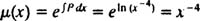
for both equations. Multiplying through by μ = x −4 yields
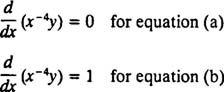
Integrating each of these resulting equations gives the general solutions:
Example 5: Sketch the integral curve of

which passes through the origin.
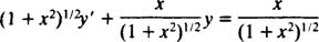
The first step is to rewrite the differential equation in standard form:
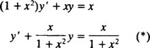
Since
the integrating factor is

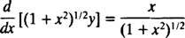
Multiplying both sides of the standard‐form equation (*) by μ = (1 + x 2) 1/2 gives
As usual, the left‐hand side collapses into (μ y)
and an integration gives the general solution:
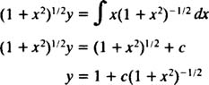
To find the particular curve of this family that passes through the origin, substitute ( x,y) = (0,0) and evaluate the constant c:

Therefore, the desired integral curve is
which is sketched in Figure 1.

Figure 1
Example 6: An object moves along the x axis in such a way that its position at time t > 0 is governed by the linear differential equation
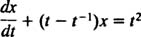
If the object was at position x = 2 at time t = 1, where will it be at time t = 3?
Rather than having x as the independent variable and y as the dependent one, in this problem t is the independent variable and x is the dependent one. Thus, the solution will not be of the form “ y = some function of x” but will instead be “ x = some function of t.”
The equation is in the standard form for a first‐order linear equation, with P = t – t −1 and Q = t 2. Since
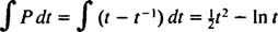
the integrating factor is

Multiplying both sides of the differential equation by this integrating factor transforms it into
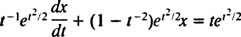
As usual, the left‐hand side automatically collapses,
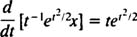
and an integration yields the general solution:
Now, since the condition “ x = 2 at t = 1” is given, this is actually an IVP, and the constant c can be evaluated:

Thus, the position x of the object as a function of time t is given by the equation
and therefore, the position at time t = 3 is
which is approximately 3.055.