First‐order equations. The validity of term‐by‐term differentiation of a power series within its interval of convergence implies that first‐order differential equations may be solved by assuming a solution of the form

substituting this into the equation, and then determining the coefficients c n .
Example 1: Find a power series solution of the form

for the differential equation

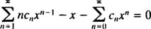
Substituting

into the differential equation yields
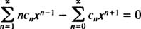
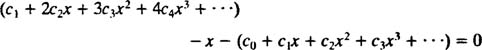
Now, write out the first few terms of each series,

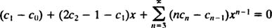
and combine like terms:

Since the pattern is clear, this last equation may be written as
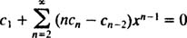
In order for this equation to hold true for all x, every coefficient on the left‐hand side must be zero. This means c 1 = 0, and for all n ≥ 2,
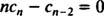
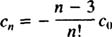
This last equation defines the recurrence relation that holds for the coefficients of the power series solution:
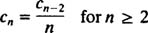
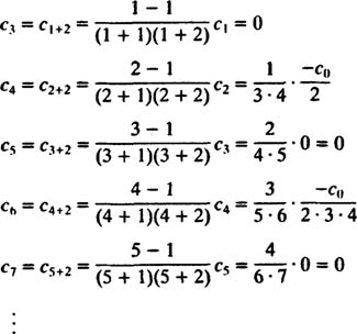
Since there is no constraint on c 0, c 0 is an arbitrary constant, and it is already known that c 1 = 0. The recurrence relation above says c 2 = ½ c 0 and c 3 = ⅓ c 1, which equals 0 (because c 1 does). In fact, it is easy to see that every coefficient c n with n odd will be zero. As for c 4, the recurrence relation says
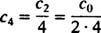
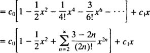
and so on. Since all c n with n odd equal 0, the desire power series solution is therefore
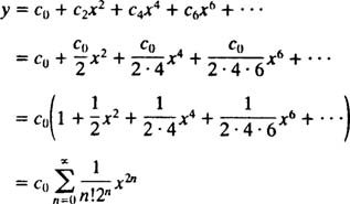
Note that the general solution contains one parameter ( c 0), as expected for a first‐order differential equation. This power series is unusual in that it is possible to express it in terms of an elementary function. Observe:
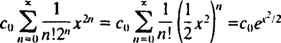
It is easy to check that y = c 0 e x2 / 2 is indeed the solution of the given differential equation, y′ = xy. Remember: Most power series cannot be expressed in terms of familiar, elementary functions, so the final answer would be left in the form of a power series.
Example 2: Find a power series expansion for the solution of the IVP

Substituting

into the differential equation yields
or, collecting all the terms on one side,
Writing out the first few terms of the series yields
or, upon combining like terms,

Now that the pattern is clear, this last equation can be written
In order for this equation to hold true for all x, every coefficient on the left‐hand side must be zero. This means

The last equation defines the recurrence relation that determines the coefficients of the power series solution:
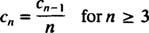
The first equation in (*) says c 1 = c 0, and the second equation says c 2 = ½(1 + c 1) = ½(1 + c 0). Next, the recurrence relation says
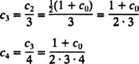
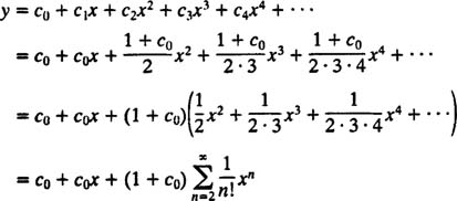
and so on. Collecting all these results, the desired power series solution is therefore
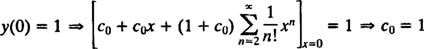
Now, the initial condition is applied to evaluate the parameter c 0:
Therefore, the power series expansion for the solution of the given IVP is
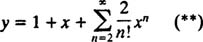
If desired, it is possible to express this in terms of elementary functions. Since
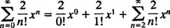
equation (**) may be written
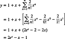
which does indeed satisfy the given IVP, as you can readily verify.
Second‐order equations. The process of finding power series solutions of homogeneous second‐order linear differential equations is more subtle than for first‐order equations. Any homogeneous second‐order linear differential equation may be written in the form 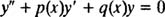
If both coefficient functions p and q are analytic at x 0, then x 0 is called an ordinary point of the differential equation. On the other hand, if even one of these functions fails to be analytic at x 0, then x 0 is called a singular point. Since the method for finding a solution that is a power series in x 0 is considerably more complicated if x 0 is a singular point, attention here will be restricted to power series solutions at ordinary points.
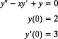
Example 3: Find a power series solution in x for the IVP
Substituting

into the differential equation yields
The solution may now proceed as in the examples above, writing out the first few terms of the series, collecting like terms, and then determining the constraints on the coefficients from the emerging pattern. Here's another method.
The first step is to re‐index the series so that each one involves x n . In the present case, only the first series must be subjected to this procedure. Replacing n by n + 2 in this series yields
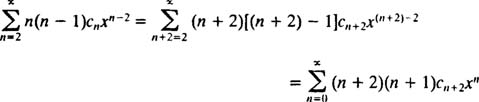
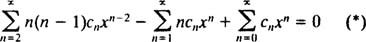
Therefore, equation (*) becomes

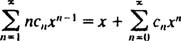
The next step is to rewrite the left‐hand side in terms of a single summation. The index n ranges from 0 to ∞ in the first and third series, but only from 1 to ∞ in the second. Since the common range of all the series is therefore 1 to ∞, the single summation which will help replace the left‐hand side will range from 1 to ∞. Consequently, it is necessary to first write (**) as

and then combine the series into a single summation:
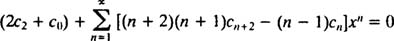
In order for this equation to hold true for all x, every coefficient on the left‐hand side must be zero. This means 2 c 2 + c 0 = 0, and for n ≥ 1, the following recurrence relation holds:
Since there is no restriction on c 0 or c 1, these will be arbitrary, and the equation 2 c 2 + c 0 = 0 implies c 2 = −½ c 0. For the coefficients from c 3 on, the recurrence relation is needed:
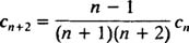
The pattern here isn't too difficult to discern: c n = 0 for all odd n ≥ 3, and for all even n ≥ 4,
This recurrence relation can be restated as follows: for all n ≥ 2,
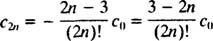
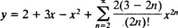
The desired power series solution is therefore
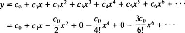
As expected for a second‐order differential equation, the general solution contains two parameters ( c 0 and c 1), which will be determined by the initial conditions. Since y(0) = 2, it is clear that c 0 = 2, and then, since y′(0) = 3, the value of c 1 must be 3. The solution of the given IVP is therefore
Example 4: Find a power series solution in x for the differential equation
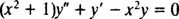
Substituting

into the given equation yields
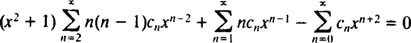
or

Now, all series but the first must be re‐indexed so that each involves x n :
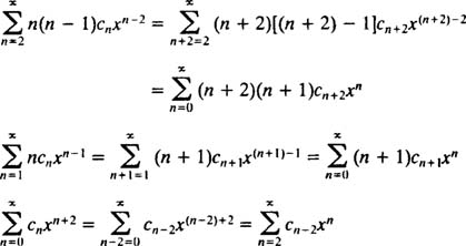
Therefore, equation (*) becomes
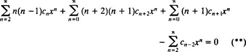
The next step is to rewrite the left‐hand side in terms of a single summation. The index n ranges from 0 to ∞ in the second and third series, but only from 2 to ∞ in the first and fourth. Since the common range of all the series is therefore 2 to ∞, the single summation which will help replace the left‐hand side will range from 2 to ∞. It is therefore necessary to first write (**) as
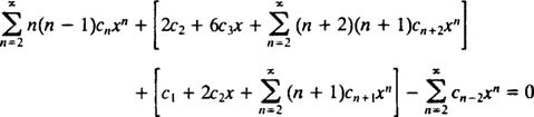
and then combine the series into a single summation:
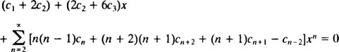
Again, in order for this equation to hold true for all x, every coefficient on the left‐hand side must be zero. This means c 1 + 2 c 2 = 0, 2 c 2 + 6 c 3 = 0, and for n ≥ 2, the following recurrence relation holds:
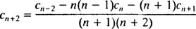
Since there is no restriction on c 0 or c 1, these will be arbitrary; the equation c 1 + 2 c 2 = 0 implies c 2 = −½ c 1, and the equation 2 c 2 + 6 c 3 = 0 implies c 3 = −⅓ c 2 = −⅓(‐½ c 1) = ⅙ c 1. For the coefficients from c 4 on, the recurrence relation is needed:
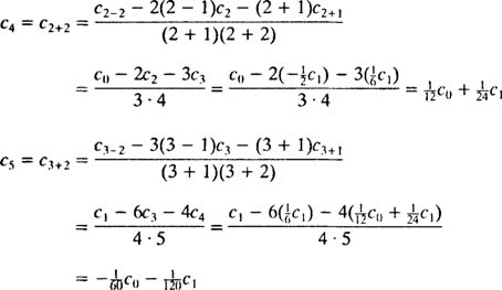
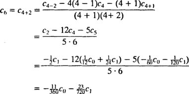
The desired power series solution is therefore

Determining a specific pattern to these coefficients would be a tedious exercise (note how complicated the recurrence relation is), so the final answer is simply left in this form.
|
|
|
|
|