For the differential equation

the method of undetermined coefficients works only when the coefficients a, b, and c are constants and the right‐hand term d( x) is of a special form. If these restrictions do not apply to a given nonhomogeneous linear differential equation, then a more powerful method of determining a particular solution is needed: the method known as variation of parameters.
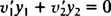
The first step is to obtain the general solution of the corresponding homogeneous equation, which will have the form
where y 1 and y 2 are known functions. The next step is to vary the parameters; that is, to replace the constants c 1 and c 2 by (as yet unknown) functions v 1( x) and v 2( x) to obtain the form of a particular solution y of the given nonhomogeneous equation:
The goal is to determine these functions v 1 and v 2. Then, since the functions y 1 and y 2 are already known, the expression above for y yields a particular solution of the nonhomogeneous equation. Combining y with y hthen gives the general solution of the non‐homogeneous differential equation, as guaranteed by Theorem B.
Since there are two unknowns to be determined, v 1 and v 2, two equations or conditions are required to obtain a solution. One of these conditions will naturally be satisfying the given differential equation. But another condition will be imposed first. Since y will be substituted into equation (*), its derivatives must be evaluated. The first derivative of y is

Now, to simplify the rest of the process—and to produce the first condition on v 1 and v 2—set
This will always be the first condition in determining v 1 and v 2; the second condition will be the satisfaction of the given differential equation (*).
Example 1: Give the general solution of the differential equation y″ + y = tan x.
Since the nonhomogeneous right‐hand term, d = tan x, is not of the special form the method of undetermined coefficients can handle, variation of parameters is required. The first step is to obtain the general solution of the corresponding homogeneous equation, y″ + y = 0. The auxiliary polynomial equation is  whose roots are the distinct conjugate complex numbers m = ± i = 0 ± 1 i. The general solution of the homogeneous equation is therefore
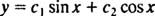
Now, vary the parameters c 1 and c 2 to obtain
Differentialtion yields

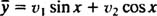
Nest, remember the first condition to be imposed on v 1 and v 2:
that is,

This reduces the expression for y′ to

so, then,

Substitution into the given nonhomogeneous equation y″ + y = tan x yields
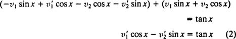
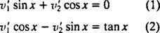
Therefore, the two conditions on v 1 and v 2 are
To solve these two equations for v 1′ and v 2′, first multiply the first equation by sin x; then multiply the second equation by cos x:
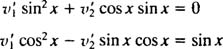
Adding these equations yields

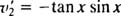
Substituting v 1′ = sin x back into equation (1) [or equation (2)] then gives
Now, integrate to find v 1 and v 2 (and ignore the constant of integration in each case):
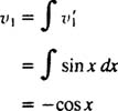
and
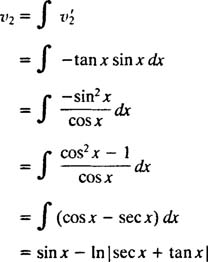
Therefore, a particular solution of the given nonhomogeneous differential equation is
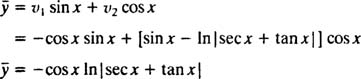
Combining this with the general solution of the corresponding homogeneous equation gives the general solution of the nonhomogeneous equation:

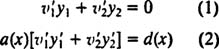
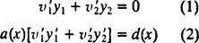
In general, when the method of variation of parameters is applied to the second‐order nonhomogeneous linear differential equation

with y = v 1( x) y 1 + v 2( x) y 2 (where y h = c 1 y 1 +c 2 y 2 is the general solution of the corresponding homogeneous equation), the two conditions on v 1 and v 2 will always be
So after obtaining the general solution of the corresponding homogeneous equation ( y h = c 1 y 1 + c 2 y 2) and varying the parameters by writing y = v 1 y 1 + v 2 y 2, go directly to equations (1) and (2) above and solve for v 1′ and v 2′.
Example 2: Give the general solution of the differential equation
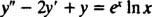
Because of the In x term, the right‐hand side is not one of the special forms that the method of undetermined coefficients can handle; variation of parameters is required. The first step requires obtaining the general solution of the corresponding homogeneous equation, y″ – 2 y′ + y = 0:

Varying the parameters gives the particular solution

and the system of equations (1) and (2) becomes
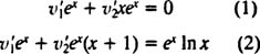
Cancel out the common factor of e x in both equations; then subtract the resulting equations to obtain

Substituting this back into either equation (1) or (2) determines

Now, integrate (by parts, in both these cases) to obtain v 1 and v 2 from v 2′ and v 2′:
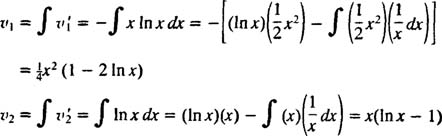
Therefore, a particular solution is
Consequently, the general solution of the given nonhomogeneous equation is

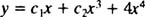
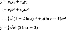
Example 3: Give the general solution of the following differential equation, given that y 1 = x and y 2 = x 3 are solutions of its corresponding homogeneous equation:
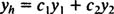
Since the functions y 1 = x and y 2 = x 3 are linearly independent, Theorem A says that the general solution of the corresponding homogeneous equation is

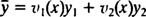
Varying the parameters c 1 and c 2 gives the form of a particular solution of the given nonhomogeneous equation:

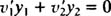
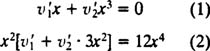
where the functions v 1 and v 2 are as yet undetermined. The two conditions on v 1 and v 2 which follow from the method of variation of parameters are
which in this case ( y 1 = x, y 2 = x 3, a = x 2, d = 12 x 4) become
Solving this system for v 1′ and v 2′ yields
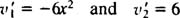
from which follow
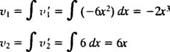
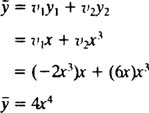
Therefore, the particular solution obtained is
and the general solution of the given nonhomogeneous equation is