The differential equation
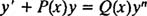
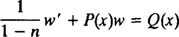
is known as Bernoulli's equation. If n = 0, Bernoulli's equation reduces immediately to the standard form first‐order linear equation:
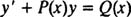
If n = 1, the equation can also be written as a linear equation:

However, if n is not 0 or 1, then Bernoulli's equation is not linear. Nevertheless, it can be transformed into a linear equation by first multiplying through by y − n ,
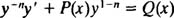
and then introducing the substitutions
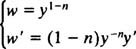
The equation above then becomes
which is linear in w (since n ≠ 1).
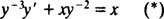
Example 1: Solve the equation

Note that this fits the form of the Bernoulli equation with n = 3. Therefore, the first step in solving it is to multiply through by y − n = y −3:
Now for the substitutions; the equations
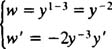
transform (*) into
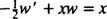
or, in standard form,

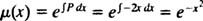
Notice that the substitutions were successful in transforming the Bernoulli equation into a linear equation (just as they were designed to be). To solve the resulting linear equation, first determine the integrating factor:
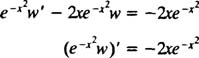
Multiplying (**) through the  yields
And an integration gives
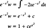
The final step is simply to undo the substitution w = y −2. The solution to the original differential equation is therefore
