First, a theorem:
Theorem O. Let A be an n by n matrix. If the n eigenvalues of A are distinct, then the corresponding eigenvectors are linearly independent.
Proof. The proof of this theorem will be presented explicitly for n = 2; the proof in the general case can be constructed based on the same method. Therefore, let A be 2 by 2, and denote its eigenvalues by λ 1 and λ 2 and the corresponding eigenvectors by v 1 and v 2 (so that A v 1 = λ 1 v 1 and A v 2 = λ 2 v 2). The goal is to prove that if λ 1 ≠ λ 2, then v 1 and v 2 are linearly independent. Assume that

is a linear combination of v 1 and v 2 that gives the zero vector; the goal is to show that the above equation implies that c 1 and c 2 must be zero. First, multiply both sides of (*) by the matrix A: 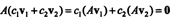
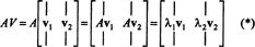
Next, use the fact that A v 1 = λ v 1 and A v 2 = λ v 2 to write

Now, multiply both sides of (*) by λ 2 and subtract the resulting equation, c 1;λ 2 v 1 + c 2λ 2 v 2 = 0 > from (**):

Since the eigenvalues are distinct, λ 1 − λ 2 ≠ 0, and since v 1 ≠ 0 ( v 1 is an eigenvector), this last equation implies that c 1 = 0. Multiplying both sides of (*) by λ 1 and subtracting the resulting equation from (**) leads to c 2(λ 2 − λ 1) v 2 = 0 and then, by the same reasoning, to the conclusion that c 2 = 0 also.
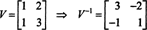
Using the same notation as in the proof of Theorem O, assume that A is a 2 by 2 matrix with distinct eigenvalues and form the matrix

whose columns are the eigenvectors of A. Now consider the product AV; since A v 1 = λ 1 v 1 and A v 2 = λ 2 v 2,
This last matrix can be expressed as the following product:
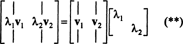
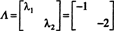
If A denotes the diagonal matrix whose entries are the eigenvalues of A,

then equations (*) and (**) together imply AV = VA. If v 1 and v 2 are linearly independent, then the matrix V is invertible. Form the matrix V −1 and left multiply both sides of the equation AV = VA by V −1:

(Although this calculation has been shown for n = 2, it clearly can be applied to an n by n matrix of any size.) This process of forming the product V −1 AV, resulting in the diagonal matrix A of its eigenvalues, is known as the diagonalization of the matrix A, and the matrix of eigenvectors, V, is said to diagonalize A. The key to diagonalizing an n by n matrix A is the ability to form the n by n eigenvector matrix V and its inverse; this requires a full set of n linearly independent eigenvectors. A sufficient (but not necessary) condition that will guarantee that this requirement is fulfilled is provided by Theorem O: if the n by n matrix A has n distinct eigenvalues.
One useful application of diagonalization is to provide a simple way to express integer powers of the matrix A. If A can be diagonalized, then V −1 AV = A, which implies

When expressed in this form, it is easy to form integer powers of A. For example, if k is a positive integer, then
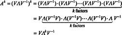
The power A k is trivial to compute: If λ 1, λ 2, …, λ n are the entries of the diagonal matrix A, then A k is diagonal with entries λ 1 k ,λ 2 k ,…, λ n k . Therefore,
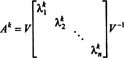
Example 1: Compute A 10 for the matrix

This is the matrix of Example 1. Its eigenvalues are λ 1 = −1 and λ 2 = −2, with corresponding eigenvectors v 1 = (1, 1) T and v 2 = (2, 3) T. Since these eigenvectors are linearly independent (which was to be expected, since the eigenvalues are distinct), the eigenvector matrix V has an inverse,
Thus, A can be diagonalized, and the diagonal matrix A = V −1 AV is
Therefore,
Although an n by n matrix with n distinct eigenvalues is guaranteed to be diagonalizable, an n by n matrix that does not have n distinct eigenvalues may still be diagonalizable. If the eigenspace corresponding to each k‐fold root λ of the characteristic equation is k dimensional, then the matrix will be diagonalizable. In other words, diagonalization is guaranteed if the geometric multiplicity of each eigenvalue (that is, the dimension of its corresponding eigenspace) matches its algebraic multiplicity (that is, its multiplicity as a root of the characteristic equation). Here's an illustration of this result. The 3 by 3 matrix

has just two eigenvalues: λ 1 = −1 and λ 2 = 3. The algebraic multiplicity of the eigenvalue λ 1 = −1 is one, and its corresponding eigenspace, E −1( B), is one dimensional. Furthermore, the algebraic multiplicity of the eigenvalue λ 2 = 3 is two, and its corresponding eigenspace, E 3( B), is two dimensional. Therefore, the geometric multiplicities of the eigenvalues of B match their algebraic multiplicities. The conclusion, then, is that although the 3 by 3 matrix B does not have 3 distinct eigenvalues, it is nevertheless diagonalizable.
Here's the verification: Since {(1, 0, −1) T} is a basis for the 1‐dimensional eigenspace corresponding to the eigenvalue λ 1 = −1, and {(0, 1, 0) T, (1, 0, 1) T} is a basis for the 2‐dimensional eigenspace corresponding to the eigenvalue λ 2 = 3, the matrix of eigenvectors reads

Since the key to the diagonalization of the original matrix B is the invertibility of this matrix, V, evaluate det V and check that it is nonzero. Because det V = 2, the matrix V is invertible,

so B is indeed diagonalizable:

Example 2: Diagonalize the matrix

First, find the eigenvalues; since
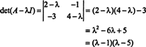
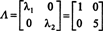
the eigenvalues are λ = 1 and λ = 5. Because the eigenvalues are distinct, A is diagonalizable. Verify that an eigenvector corresponding to λ = 1 is v 1 = (1, 1) T, and an eigenvector corresponding to λ = 5 is v 2 = (1, −3) T. Therefore, the diagonalizing matrix is
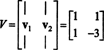
and
Another application of diagonalization is in the construction of simple representative matrices for linear operators. Let A be the matrix defined above and consider the linear operator on R 2 given by T( x) = A x. In terms of the nonstandard basis B = { v 1 = (1, 1) T, v 2 = (1, −3) T} for R 2, the matrix of T relative to B is A.